Two sets are named disjoint sets if they have no elements in common. A Disjoint-Sets (or Union-Find) data structure keeps track of a fixed number of elements partitioned into a number of disjoint sets. The data structure has two operations:
- connect(x, y): connect x and y. Also known as union
- isConnected(x, y): returns true if x and y are connected (i.e. part of the same set).
public interface DisjointSets {
    /** connects two items P and Q */
    void connect(int p, int q);

    /** checks to see if two items are connected */
    boolean isConnected(int p, int q);
}Using a single array of integers.
- The indices of the array represent the elements of our set.
- The value at an index is the set number it belongs to.
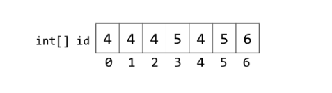
- Constructor:
$\Theta (N)$ - Connect:
$\Theta (N)$ - IsConnect:
$\Theta (1)$
Using a tree to represent it. But There is a potential performance issue with QuickUnion: the tree can become very long.
- Constructor:
$\Theta (N)$ - Connect:
$O (N)$ - IsConnect:
$O (N)$
Improving on Quick Union relies on a key insight: whenever we call find, we have to climb to the root of a tree. Thus, the shorter the tree the faster it takes!
New rule: whenever we call connect, we always link the root of the smaller tree to the larger tree.
Following the above rule ensures that the maximum height of any tree is
- Constructor:
$\Theta (N)$ - Connect:
$\Theta (log N)$ - IsConnect:
$O (log N)$
Recall that both connect(x, y) and isConnected(x, y) always call find(x) and find(y). Thus, after calling connect or isConnected enough, essentially all elements will point directly to their root.
By extension, the average runtime of connect and isConnected becomes almost constant in the long term!
- Constructor:
$\Theta (N)$ - Connect:
$o (N)$ - IsConnect:
$O (N)$
Definition: A binary search tree (BST) is a binary tree where each node has a Comparable key (and an associated value) and satisfies the restriction that the key in any node is larger than the keys in all nodes in that node's left subtree and smaller than the keys in all nodes in that node's right subtree.
We define a inner private class to define nodes in BST. Each node contains a key, a value, a left link, a right link, and a node count. The left link points to a BST for items with smaller keys, and the right link points to a BST for items with larger keys. The instance variable N gives the node count in the subtree rooted at the node.
The running times of algorithms on binary search trees depend on the shapes of the trees, which, in turn, depends on the order in which keys are inserted.
- Search(get): Find the value of Key key.
$2 lnN ~ 1.39lgN$ - Insert(put): Find the key and update it, if not make a new node.
$2 lnN ~ 1.39lgN$
Order-based methods and deletion. An important reason that BSTs are widely used is that they allow us to keep the keys in order. As such, they can serve as the basis for implementing the numerous methods in our ordered symbol-table API.
- Minimum(min) and maximum: Return the minimum/maximum of the tree
- Floor(floor) and ceiling(ceil): Find the largest key in the BST less than or equal to key
- Selection(select): Seek the key of rank k (the key such that precisely k other keys in the BST are smaller).
- rank: return the rank of Key key.
- Delete the minimum and maximum: Delete the minimum of the tree.
- Delete: For a node has two children, is to delete a node x by replacing it with its successor. In four steps.
- Save a link to the node to be deleted in t
- Set x to point to its successor min(t.right).
- Set the right link of x (which is supposed to point to the BST containing all the keys larger than x.key) to deleteMin(t.right), the link to the BST containing all the keys that are larger than x.key after the deletion.
- Set the left link of x (which was null) to t.left (all the keys that are less than both the deleted key and its successor).
- Range Search: Return keys, between low, and high
We introduce in this section a type of binary search tree where costs are guaranteed to be logarithmic. Our trees have near-perfect balance, where the height is guaranteed to be no larger than 2 lg N.
The primary step to get the flexibility that we need to guarantee balance in search trees is to allow the nodes in our trees to hold more than one key.
- The key of 2-3 tree can keep balance is that it grows from bottom to up.
Definition: A 2-3 search tree is a tree that either is empty or:
- A 2-node, with one key (and associated value) and two links, a left link to a 2-3 search tree with smaller keys, and a right link to a 2-3 search tree with larger keys
- A 3-node, with two keys (and associated values) and three links, a left link to a 2-3 search tree with smaller keys, a middle link to a 2-3 search tree with keys between the node's keys and a right link to a 2-3 search tree with larger keys.
However, we are only part of the way to an implementation. Although it would be possible to write code that performs transformations on distinct data types representing 2- and 3-nodes, most of the tasks that we have described are inconvenient to implement in this direct representation.
Encoding 3-nodes. The basic idea behind red-black BSTs is to encode 2-3 trees by starting with standard BSTs (which are made up of 2-nodes) and adding extra information to encode 3-nodes. We think of the links as being of two different types: red links, which bind together two 2-nodes to represent 3-nodes, and black links, which bind together the 2-3 tree. Specifically, we represent 3-nodes as two 2-nodes connected by a single red link that leans left. We refer to BSTs that represent 2-3 trees in this way as red-black BSTs.
Definition:
- All the red links are the left links.
- There is not a node which has two red links.
- The Reb-black tree is black balance binary tree.
Proposition: The height of a red-blackBST with N nodes is no more than 2 lg N.
Proposition: In a red-black BST, the following operations take logarithmic time in the worst case: search, insertion, finding the minimum, finding the maximum, floor, ceiling, rank, select, delete the minimum, delete the maximum, delete, and range count.
Property: The average length of a path from the root to a node in a red-black BST with N nodes is ~1.00 lg N.
If keys are small integers, we can use an array to implement a symbol table, by interpreting the key as an array index so that we can store the value associated with key i in array position i. In this section, we consider hashing, an extension of this simple method that handles more complicated types of keys. We reference key-value pairs using arrays by doing arithmetic operations to transform keys into array indices.
Search algorithms that use hashing consist of two separate parts. The first step is to compute a hash function that transforms the search key into an array index. Ideally, different keys would map to different indices. This ideal is generally beyond our reach, so we have to face the possibility that two or more different keys may hash to the same array index. Thus, the second part of a hashing search is a collision-resolution process that deals with this situation.
- Java conventions. Java helps us address the basic problem that every type of data needs a hash function by requiring that every data type must implement a method called hashCode() (which returns a 32-bit integer). The implementation of hashCode() for an object must be consistent with equals. That is, if a.equals(b) is true, then a.hashCode() must have the same numerical value as b.hashCode(). If the hashCode() values are the same, the objects may or may not be equal, and we must use equals() to decide which condition holds.
- Converting a hashCode() to an array index. Since our goal is an array index, not a 32-bit integer, we combine hashCode() with modular hashing in our implementations to produce integers between 0 and M-1 as follows:
The code masks off the sign bit (to turn the 32-bit integer into a 31-bit nonnegative integer) and then computing the remainder when dividing by M, as in modular hashing.
private int hash(Key key) {
   return (key.hashCode() & 0x7fffffff) % M;
}
- Assumption J (uniform hashing assumption). The hash function that we use uniformly distributes keys among the integer values between 0 and M-1.
- Hashing with separate chaining. A hash function converts keys into array indices. The second component of a hashing algorithm is collision resolution: a strategy for handling the case when two or more keys to be inserted hash to the same index. A straightforward approach to collision resolution is to build, for each of the M array indices, a linked list of the key-value pairs whose keys hash to that index. The basic idea is to choose M to be sufficiently large that the lists are sufficiently short to enable efficient search through a two-step process: hash to find the list that could contain the key, then sequentially search through that list for the key.
- Hashing with linear probing. Another approach to implementing hashing is to store N key-value pairs in a hash table of size M > N, relying on empty entries in the table to help with with collision resolution. Such methods are called open-addressing hashing methods. The simplest open-addressing method is called linear probing: when there is a collision (when we hash to a table index that is already occupied with a key different from the search key), then we just check the next entry in the table (by incrementing the index). There are three possible outcomes:
- every type of key needs a good hash function
- the performance depends on hash function.
- the computation of hash function may be expensive
- it is hard to support sequential data.