
Python-based post-processing PIV data analysis in the repo: https://github.com/openpiv/pivpy


Merging the three packages:
- https://github.com/tomerast/Vecpy
- https://github.com/alexlib/pivpy/tree/xarray
- https://github.com/ronshnapp/vecpy
Recommended: use uv (fast, reproducible)
Create a virtualenv and install:
uv venv
uv pip install pivpy
Install this repository (editable / development install):
uv venv
uv pip install -e .
Install with optional dependencies (including lvpyio for LaVision VC7):
uv pip install 'pivpy[full]'
Run in a sandbox (isolated) environment (no persistent venv required):
uv run --isolated --with pivpy python -c "import pivpy; print(pivpy.__version__)"
Or run with optional dependencies in the sandbox:
uv run --isolated --with "pivpy[full]" python -c "from pivpy import io; print(io)"
Run using a specific Python version (uv-managed) in the sandbox:
uv python install 3.14
uv run --isolated --managed-python -p python3.14 --with pivpy python -c "import sys, pivpy; print(sys.version.split()[0], pivpy.__version__)"
Run this repository's tests on Python 3.14 (sandboxed):
uv run --isolated --managed-python -p python3.14 --with-editable . pytest -q
Alternative: use pip:
pip install pivpy
or with optional dependencies:
pip install 'pivpy[full]'
if you use OpenPIV, PIVlab, etc.
Quick start (auto-detect file format):
from pivpy import io
ds = io.read_piv('your_file.vec')
Load experimental PIV data or generate analytical flow fields, and visualize publication-quality flow fields with zero effort:
import matplotlib.pyplot as plt
import pivpy.pivpy  # registers the .piv accessor
from pivpy import synthetic

# 1. Generate an analytical multi-vortex 2D turbulence field (or use io.read_piv)
ds = synthetic.multivortex(n_frames=1, n=128, n_vortices=8, two_d=True, seed=42)

# 2. Zero-effort, publication-quality plot (vorticity background, streamlines & auto-scaled vectors)
fig, ax = ds.piv.plot()
plt.show()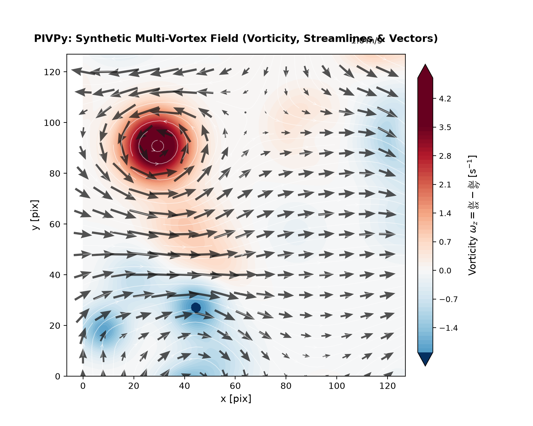
Animate time-series datasets with in-place vector updates (set_UVC) and dynamic vorticity tracking:
# 1. Generate or load time-series flow data (e.g. interacting vortex pair)
ds = synthetic.vortex_pair(n_frames=24, n=128)

# 2. Animate with one call
anim = ds.piv.animate(interval=80)

# Save as GIF / MP4 or display in Jupyter / Marimo
anim.save("vortex_interaction.gif")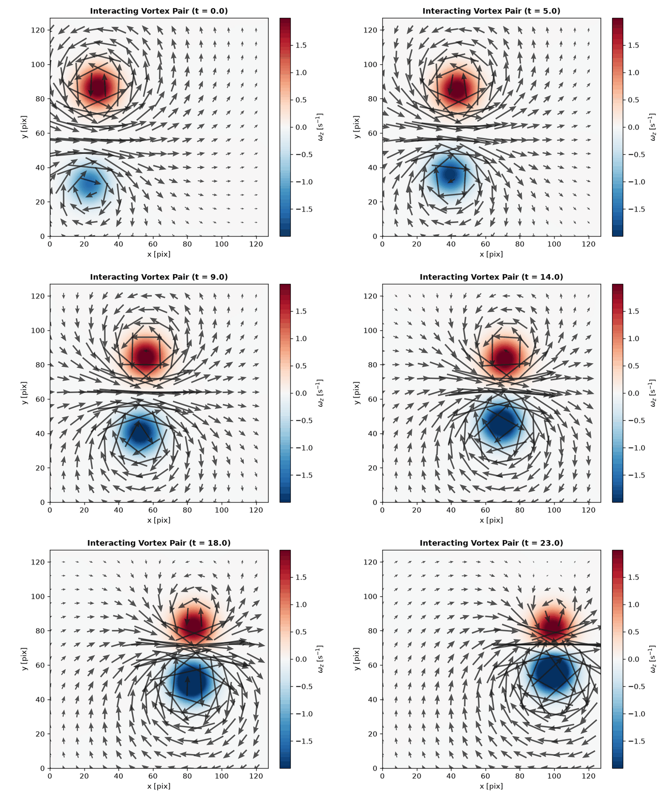
Every visual layer can be easily tailored or toggled:
# Velocity magnitude background with vectors only (no streamlines)
fig, ax = ds.piv.plot(
    background="mag",       # 'vorticity' (default), 'mag', 'ke', 'divergence', or None
    streamlines=False,      # toggle flow streamlines
    quiver=True,            # toggle velocity vectors
    blur=1.5,               # smooth fluid color gradient
    arrow_scale=0.75,       # custom vector arrow scale
    title="Velocity Magnitude & Vectors",
)

# Clean vector quiver only (no background)
fig, ax = ds.piv.plot(background=None)
Legacy loaders (still supported):
ds = io.load_vec('your_file.vec')
ds = io.load_openpiv_txt('your_file.txt')
Check whether a newer version is available on PyPI:
import pivpy
res = pivpy.check_update(verbose=True)
# res.status: 0=unavailable, 1=up-to-date, 2=update available, 3=installed newer
PIVPy exposes many post-processing operations via the xarray accessor Dataset.piv.
Several common PIVMat toolbox methods are available with similar names/behavior:
import pivpy.pivpy  # registers the .piv accessor
from pivpy import io

ds = io.create_sample_Dataset(n_frames=10)

# Add noise (similar to PIVMat addnoisef)
ds_noisy = ds.copy().piv.addnoisef(eps=0.1, opt='add', nc=0.0, seed=0)

# Ensemble (temporal) average and optional std/rms (similar to PIVMat averf)
avg = ds.piv.averf()
avg, std, rms = ds.piv.averf(return_std_rms=True)

# Spatial averages (similar to PIVMat spaverf)
ds_xy = ds.piv.spaverf('xy')   # excludes zeros by default
ds_x0 = ds.piv.spaverf('x0')   # include zeros

# Subtract ensemble/spatial average (similar to PIVMat subaverf)
fluct = ds.piv.subaverf('e')
fluct_x = ds.piv.subaverf('x0')

# Azimuthal averaging (similar to PIVMat azaverf)
r, ur, ut = ds.isel(t=0).piv.azaverf(0.0, 0.0, return_profiles=True)

# Temporal resampling and phase average (similar to PIVMat resamplef/phaseaverf)
ds_r = ds.piv.resamplef(tini=range(ds.sizes['t']), tfin=[0.5, 1.5, 2.5])
phased = ds.piv.phaseaverf(12)
Additional PIVMat-inspired utilities:
# Correlation along a dimension (similar to PIVMat corrm/corrx)
cu = ds.piv.corrm(variable='u', dim='x')        # returns DataArray with a 'lag' dimension
cv = ds.piv.corrm(variable='v', dim='y', half=True)

# Spatial correlation function + integral scales (similar to PIVMat corrf)
cor = ds.piv.corrf(variable='u', dim='x', normalize=True)
# correlation curve: cor['f'] over cor['r']
# integral scales: cor['isinf'], cor['is5'], cor['is2'], cor['is1'], cor['is0']

# Fill holes encoded as zeros (similar to PIVMat interpolat.m behavior)
ds_filled = ds.piv.fill_zeros(max_iter=10)

# Extract a rectangular region (similar to PIVMat extractf)
sub = ds.piv.extractf([0.0, 0.0, 10.0, 5.0], 'phys')   # [x1,y1,x2,y2] in physical units
sub = ds.piv.extractf([10, 5, 50, 40], 'mesh')         # 1-based mesh indices (MATLAB-like)

# Spatial convolution filter (similar to PIVMat filterf)
ds_smooth = ds.piv.filterf(1.0, 'gauss', 'same')   # keep same size
ds_smooth_valid = ds.piv.filterf(1.0, 'gauss')     # smaller (conv2(...,'valid') behavior)

# Flip field (similar to PIVMat flipf)
ds_lr = ds.piv.flipf('x')     # left-right mirror (negates u)
ds_tb = ds.piv.flipf('y')     # top-bottom mirror (negates v)
ds_xy = ds.piv.flipf('xy')    # both

# 2D Butterworth filter (similar to PIVMat bwfilterf)
ds_low = ds.piv.bwfilterf(filtsize=3.0, order=8.0, mode='low', trunc=True)
ds_high = ds.piv.bwfilterf(filtsize=3.0, order=8.0, mode='high')

# PIVMat-style option wrapper: opts can include 'high'/'low'/'trunc'
ds_high2 = ds.piv.bwfilterf_pm(3.0, 8.0, 'high', 'trunc')

# Batch processing over filename series (similar to PIVMat batchf)
# fun can be a callable (fun(ds, ...)) or an accessor method name (e.g. 'averf', 'bwfilterf')
from pivpy.io import batchf
results = batchf('pivpy/data/day2/day2a00500[0:5].T000.D000.P003.H001.L.vec', 'averf')
Using uv (recommended):
git clone https://github.com/alexlib/pivpy .
cd pivpy
uv venv
uv pip install -e .
Editable install with optional dependencies:
uv pip install -e '.[full]'
Alternative (conda):
git clone https://github.com/alexlib/pivpy .
cd pivpy
conda create -n pivpy python=3.11
conda activate pivpy
conda install pip
pip install -e .
-
lvpyioby Lavision Inc. if you use vc7 files -
netcdf4if you want to store NetCDF4 files by xarray -
pyarrowif you want to store parquet files -
vortexfittingif you want to do vortex analysis ($\lambda_2$ and$Q$ criterions, vortex fitting) -
numpy,scipy,matplotlib,xarrayare must and installed with thepivpy
- @alexlib
- @ronshnapp - original steps
- @liorshig - LVreader and great visualizaiton for Lavision
- @nepomnyi - connection to VortexFitting and new algorithms
Look into the getting started marimo notebook
(open it with uv run marimo edit examples/notebooks/Getting_Started.py, or click the
"Open in molab" badge above to run it in your browser)
and additional notebooks: Notebooks
From a command line just use:
pytest
With uv:
uv run pytest -q
Read the ToDo file and pick one item to program. Use Fork-Develop-Pull Request model to contribute
Tutorials live as marimo notebooks (.py files) in docs/source/. The Sphinx build
(docs/source/conf.py) exports them to static HTML via marimo export html and embeds them
in the generated docs automatically -- no separate conversion step needed:
uv pip install -r docs/requirements.txt
uv run sphinx-build -b html docs/source/ docs/build/html
generates docs/build/html directory with the documentation